This C++/ROOT software was created by Sara Gamba and Giulia Nigrelli for the Computing Methods for Experimental Physics and Data Analysis exam.
Introduction
Using MC and Run datas of the dimuon events of CMS, the main goals of this software are essentially three:
- the measurement of the Z resonance;
- the measurement of the angle of the negative muon in the Collins–Soper frame of the dimuon system;
- the measurement of the forward-backward asymmetry.
This functionalities are built in order to recreate similar plots of the article
Measurement of the weak mixing angle using the forward-backward asymmetry of Drell–Yan events in pp collisions at 8 TeV by the CMS collaboration.
For simplifying the usage, a main is provided in order to execute the program.
Requirements
- CERN ROOT 6.26
- Python3
An example of usage
The whole project is done in C++ files, but the compilation is done with python. You can type in the terminal, in the main "cmepdaexam" folder:
You can have some options:
You have to choose (the filter option is mandatory) if you want to filter your datas or not. In the first case:
In this case you have to write also:
For example we chose file from here:
The program will accept only files that exist and that have the right columns, if there aren't the program will stop. Then you have to choose the name of your filtered dataframes files. Be careful: you have to put the .root extension to your filtered files or you won't be able to use them. In this case you have to choose only file name already filtered:
If you have already used the filter function for one of the analysis and you don't want to repeat it, you can choose to not filter your datas:
Then you have to choose the name of your filtered dataframes files. Be careful: you have to put the .root extension to your filtered files or you won't be able to use them. In this case you have to choose only file name already filtered:
Then you have to insert which analysis you want to do, with this option:
You can choose between:
- cos: the measurement of the angle of the negative muon in the Collins–Soper frame of the dimuon system;
- dimspec: the measurement of the Z resonance;
- afb: the measurement of the forward-backward asymmetry;
- 0: quit.
After the analysis the program will stop. If your analysis well ended, you can find your plots on the directory "images".
The default applied filters are on the following columns of the dataframes:
- nMuon;
- Muon_charge;
- Muon_eta;
- Muon_pt;
- Muon_dxy;
- Muon_pfRelIso03_chg.
Description of main (and functionality of libraries)
Filter function
The filter function is the first function we have to use. It has the main target to filter the CMS Open Data. We have 100GB of MC events and almost 100GB of Run events. We have to filter them, as said before, with this filters:
- number of muons equal to 2;
- the product of the first muon charge and the second is equal to -1;
- the two pseudorapidities are less than 2.4;
- The \(Muon_{first,pt}\) is greater than 25 and \(Muon_{second,pt}\) is greater than 15 or vice versa;
- the transverse distance of the two muons is less than 0.2;
- the muon isolation is less than 10% of \(Muon_{pt}\).
The Dataset of MC datas and Run datas are saved through two Snapshots of the Dataframes with new useful variables:
- \(Muon_{pt}\): Trasversal momentum of the two muons;
- \(Muon_{eta}\): Pseudorapidity of the two muons;
- \(Muon_{phi}\): Coordinate phi of the two muons;
- \(Muon_{mass}\): Mass of the muons.
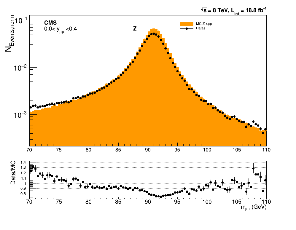
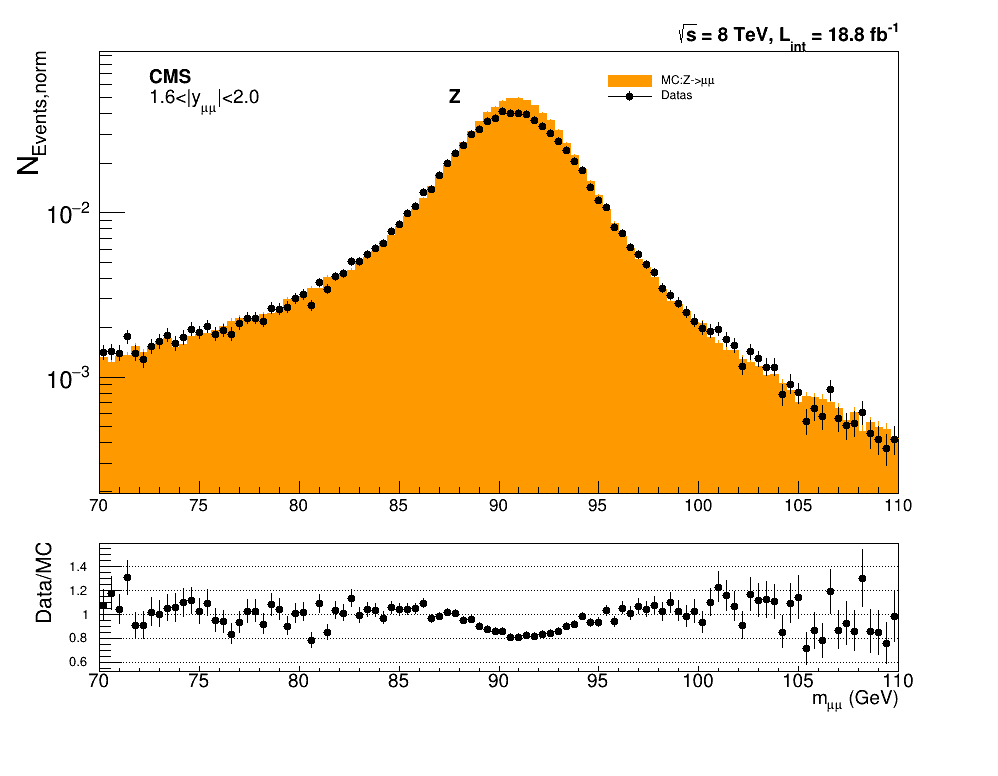
Dimuon mass Spectrum of Z
This macro will do the normalized histograms of the dimuon mass Spectrum of Z. First it will be created a column of the dimuon four vector, passing the four column we have saved to the function in utilities.h that returns the four vector of the dimuon system. Then we will calculate the dimuon invariant mass. We have also calculated the rapidity in order to plot three different plots with different costraints of rapidity. The MC datas will be plotted in yellow and the Run datas will be plotted as black points. We normalized the histograms with the total number of the events of MC and Run datas.
The canvas is saved in the directory images and in the subdirectory dimuonspectrumZ as dimuon_spectrum_Zi.pdf and dimuon_spectrum_Zi.png, where \(i\) is the costraints of rapidity. If the directories don't exist, then the program will create them.
We report our dimuon mass spectrum of Z particle with different costraints of rapidity. In this pictures we have the yellow histogram that represent the MC datas, and the black point the Run datas. The low histogram is the ratio between the other two. All the histogram are normalized with the total number of events.

A more detail description of the functions used it can be found in dimuonSpectrumZ.h, utilities.h and graphicalUtilities.h.
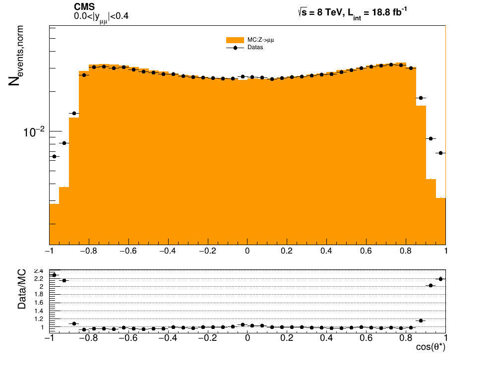
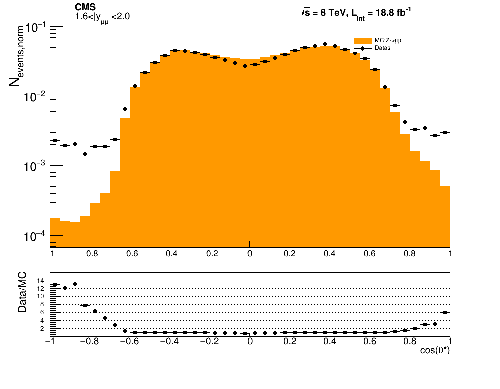
cos(theta*)
This macro will do the normalized histograms of the angle of the negative muon in the Collins–Soper frame of the dimuon system. First it will be created three columns of the dimuon four vector, first muon four vector and second muon four vector, passing the four column we have saved to the function in utilities.h. Then we will calculate the dimuon invariant mass and other quantities foundamental to calculate \(cos(\theta^*)\). We have also calculated the rapidity in order to plot three different plots with different costraints of rapidity. The MC datas will be plotted in yellow and the Run datas will be plotted as black points. We normalized the histograms with the total number of the events of MC and Run datas.
The canvas is saved in the directory images and in the subdirectory costheta as costhetai.pdf and costhetai.png, where \(i\) is the costraints of rapidity. If the directories don't exist, then the program will create them.
We report our measurement of the angle of the negative muon in the Collins–Soper frame of the dimuon system with different costraints of rapidity. In this pictures we have the yellow histogram that represent the MC datas, and the black point the Run datas. The low histogram is the ratio between the other two. All the histogram are normalized with the total number of events.

A more detail description of the functions used it can be found in costheta.h , utilities.h and graphicalUtilities.h.
Afb
This macro will do the 2D histogram of Afb in function of dimuon mass of MC events and of RUN events. First it will be created three columns of the dimuon four vector, first muon four vector and second muon four vector, passing the four column we have saved to the function in utilities.h. Then we will calculate the dimuon invariant mass and other quantities foundamental to calculate \(cos(\theta^*)\), \(wd\) and \(wn\) (variables you can find in the article). We have also calculated the rapidity in order to plot six different plots in one canvas with different costraints of rapidity. The MC datas will be plotted as black points.
The canvas is saved in the directory images and in the subdirectory afb as afb.pdf and afb.png, If the directories don't exist, then the program will create them.
A more detail description of the functions used it can be found in afb.h , utilities.h and graphicalUtilities.h.
We report our measurement of the asymmetry forward backward. We have drawn only th MC events.

Testing
We have done tests in C++, but the compilation is done with python. You can type in the terminal, in the main "cmepdaexam" folder:
You can have some options:
You have to choose (the filter option is mandatory only for tests 2, 3, 4) if you want to filter your datas or not. In the first case:
In this case you have to write also:
For example we chose file from here:
The program will accept only files that exist and that have the right columns, if there aren't the program will stop. Then you have to choose the name of your filtered dataframes files. Be careful: you have to put the .root extension to your filtered files or you won't be able to use them. In this case you have to choose only file name already filtered:
If you have already used the filter function for one of the analysis and you don't want to repeat it, you can choose to not filter your datas:
Then you have to choose the name of your filtered dataframes files. Be careful: you have to put the .root extension to your filtered files or you won't be able to use them. In this case you have to choose only file name already filtered:
Then you have to insert which test you want to do, with this option:
If you want to do test 5 or 1 it is not necessary to write the filter option. You can only put the testopt.
You will be able to choose the test you want to do:
- 1: test on filter function;
- 2: test on costheta value;
- 3: test on energy value;
- 4: test on energy formula value;
- 5: test on operation histograms.
After a test your program will stop. If the test well ended there will be written "Test passed!". The default applied filters are on the following columns of the dataframes:
- nMuon;
- Muon_charge;
- Muon_eta;
- Muon_pt;
- Muon_dxy;
- Muon_pfRelIso03_chg.
Test on filter function
Test on filter function handles the correct error given by the filter function. In this test we call filterDf(), with wrong path, empty dataframe, right dataframe, dataframe with few columns to see if the error given by the function corresponds to our previsions. It prints "Test passed!" everything was done correctly or "Test failed!". A more detail description of the functions used it can be found in testFilt.cpp.
Test on costheta value
Test on costheta function handles if \(|cos(\theta^*)|\), defined in utilities.h, is <1. It creates all quantities in allquantities() and we check how many rows left with \(|cos(\theta^*)|>1\). It prints "Test passed!" if there are no rows left or "Test failed!". A more detail description of the functions used it can be found in testCos.cpp.
Test on energy value
Test on energy values function handles if \(E_1+E_2-E_{tot}\), defined in utilities.h, is less or higher than 0.01% of \(E_{tot}\). It creates all quantities in allquantities() and we check how many rows left with \(|E_1+E_2-E_{tot}|>0.01\)% \(E_{tot}\). It prints "Test passed!" if there are no rows left or "Test failed!". A more detail description of the functions used it can be found in testEnergy.cpp.
Test on energy value formulas
Test on energy values function handles if \(E_i^2=p_i^2+m^2\), defined in utilities.h, is less or higher than 0.01% of \(E_i\). It creates all quantities in allquantities() and we check how many rows left with \(|E_i-(p_i^2+m^2)|>0.01\)% \(E_i\). It prints "Test passed!" if there are no rows left or "Test failed!". A more detail description of the functions used it can be found in testEnergyFormulas.cpp.
Test on operation histograms
Test on operationHist() function handles if the operations done on 4 different histograms have the correct result. It creates four histograms and then four random variables. We have inserted the variables in four different bins of the four histograms, rearranged to create new variables. Then we have test if the difference between the content of each bin and the variable calculated ( \(var_{calc}\)) as we expect is < 0.01% \(var_{calc}\). Then the program checks if the content of each bin and the variable calculated are concord. It prints "Test passed!" if the statements are true or "Test failed!" if not. A more detail description of the functions used it can be found in testOperationHist.cpp.